For loops
This workshop is going to go through the different ways of writing and implementing for loops in R. From subsetting your data into different chunks, to generating individuals plots, to bootstrapping iterations, hopefully by the end of this workshop you’ll be able to implement loops into your code and make it more efficient and less frustrating. We will also cover how to include if else statements into your code.
Now, many of these examples can be done using the apply family or the purrr package, but it sounds like the apply family is starting to get phased out. The purrr package is more tidyverse-friendly as it allows for %>%, but in many instances it would require you to also write out your own function(), even if it uses a predetermined function. So, for the purpose of this workshop, we’ll stick to for() loops.
What are for loops?
For loops are basically a way of repeating a task (or a series of tasks) over and over again. If you have ever had to copy-paste a chunk of code more that two times, then you would have probably been better off using a for loop.
Why do we need for loops?
Great question! As much fun as it is to copy-paste something 10000000000 times, it can introduce some problems.
- What if you wanted to change a single element and apply it to everything? Now you have to rewrite the same line over and over and over again, which can very easily introduce mistakes that are hard to catch
- For loops run iteratively, so you can just hit “run” and let it go! This saves you a bunch of time instead of running one iteration, waiting for it finish, then running the next and so on.
- It’s more reproducible-friendly. Nobody wants to go through your 39485728059824375 lines of code, especially if you have the same 200 lines repeating
Long story short, if you have ever had to copy-paste something a bunch of times, you were probably better off writing it into a loop. Of course, they are not obviously intuitive, but once you get the hang of it, you’ll love running them!
From this workshop, we’ll start off with some very easy and basic for loops, then we’ll get into some more everyday examples of when they’re useful, and we’ll end the workshop with some not-so-complicated nested for loops (i.e. a loop within a loop).
Basic loops
In this section, we’ll go through the very basics of a for loop and how they are typically coded. We call them “for loops” because we’re telling the computer “for every element in my list, do this task”. So, if we had a list of names and we wanted to print them, we’d say “for every name in my list, print it”
for (name in c('Isabelle', 'Juliano', 'Will')) print(name)
## [1] "Isabelle"
## [1] "Juliano"
## [1] "Will"
We can give it the list inside the parentheses, or we can specify a list outside of the loop and then feed it in
name_list <- c('Isabelle', 'Juliano', 'Will')

for (name in name_list) print(name)
## [1] "Isabelle"
## [1] "Juliano"
## [1] "Will"
We end up with the same outcome! This will be very helpful down the road when lists get longer.
You’ll notice that the function, in this case
print(), came immediately after the
for() call. That’s because we are
only asking it to do a single function (in this case
print()). If you want it to perform
multiple functions, then you will need to add curly brackets {}
for (name in name_list) {

  name2 <- paste(name, 'rocks at coding!', sep = ' ')
  print(name2)

}
## [1] "Isabelle rocks at coding!"
## [1] "Juliano rocks at coding!"
## [1] "Will rocks at coding!"
In this example, we’ve created a second object called name2, where we
added a pasted phrase of ‘rocks at coding’ and separated clauses with a
space. Now, the important thing to note here is that each time the loop
runs through an iteration, it is rewriting what name2 is. That means
that when the loop is finished, name2 will take on the last value of
the list.
name2
## [1] "Will rocks at coding!"
This means that we did not keep any of the previous versions of name2.
What if we want access to all three? That’s where things get exciting.
We’ll have to designate an empty list outside the loop, and then
assign values to things from the loop.
# first, create an empty list that we will infill later
name2_list <- list()

# Now, we'll run the loop and assign each value to its own element from the list
for (name in name_list) {

  name2 <- paste(name, 'rocks at coding!', sep = ' ') # create the statement
  print(name2) # print it out to read
  name2_list[[name]] <- name2 # assign it to the list

}
## [1] "Isabelle rocks at coding!"
## [1] "Juliano rocks at coding!"
## [1] "Will rocks at coding!"
We assign objects in the list using the double square brackets [[]].
Under the hood, R converts the character string that you feed it
(i.e. name) into numeric.
Now, we can pull out individual values from the list we created
name2_list[[1]]
## [1] "Isabelle rocks at coding!"
name2_list[[2]]
## [1] "Juliano rocks at coding!"
Groovy! Ok, so we’ve assigned ‘rocks at coding!’ to everyone, but what if we wanted to say something different about Juliano? That’s when we can use if else statements. An if else statement is basically telling R “If the element of the list is equal to a specific value, do this task. For everything else, do this other task”.
for (name in name_list) {

  # We'll start with the condition if the name is Juliano
  if (name == 'Juliano')
    name2 <- paste(name, 'is amazing at coding!', sep = ' ')
  # for everything else in the list
  else
    name2 <- paste(name, 'rocks at coding!', sep = ' ')

  print(name2)

}
## [1] "Isabelle rocks at coding!"
## [1] "Juliano is amazing at coding!"
## [1] "Will rocks at coding!"
Just like the for() statement before, because we only have a single function in our if else statement, we don’t need curly brackets. If we had multiple functions, we would add curly brackets. We’ll go through some more complicated examples below.
Now, what if we wanted to say something different about each name? Then we would add more if statements in:
for (name in name_list) {

  # We'll start with the condition for Juliano
  if (name == 'Juliano')
    name2 <- paste(name, 'is amazing at coding!', sep = ' ')
  # Now we'll change it for Isabelle too
  else if (name == 'Isabelle')
    name2 <- paste(name, 'is super cool!', sep = ' ')
  # Now the last one left will take the else statement
  else
    name2 <- paste(name, 'rocks at coding!', sep = ' ')

  print(name2)

}
## [1] "Isabelle is super cool!"
## [1] "Juliano is amazing at coding!"
## [1] "Will rocks at coding!"
You can layer as many if statements onto your block as you want. We’ll go through some examples below of how this can make things easier.
Ok, what if we actually didn’t want to say anything about Juliano at all? What if we wanted to skip Juliano? Then we can use the command next. We would use it inside an if statement block and basically tell R “If the element of the list is equal to a specific value, move on to the next element”.
for (name in name_list) {

  # We'll tell the for loop to move to the next value after Juliano
  if (name == 'Juliano') next

  # Create our name2 object and print it
  name2 <- paste(name, 'is amazing at coding!', sep = ' ')
  print(name2)

}
## [1] "Isabelle is amazing at coding!"
## [1] "Will is amazing at coding!"
In this example, we don’t need to specify an else portion to the if statement, because it knows to just move onto the next value. This can become very helpful when you’re iterating through a list of values in a dataframe and you just want to skip one (or multiple) levels. It will save you from having to create a whole separate dataframe or rewriting out an entire list and omitting those specific levels.
We can also tell the loop to break at
a certain value. This is helpful when you’re generating a big loop and
you want to troubleshoot any problems that you might have. For example,
you can tell R things like “If an
error occurs with this iteration,
break the loop”. It’s also helpful in
cases if, say, you want rows n and n+1 from a dataframe. When you
get to the last row, then there is no more n+1, so you can tell the
loop to break.
for (name in name_list) {

  # We'll tell the loop to break at Juliano
  if (name == 'Juliano') break

  # Create the name2 object and print it
  name2 <- paste(name, 'is amazing at coding!', sep = ' ')
  print(name2)

}
## [1] "Isabelle is amazing at coding!"
Some things to keep in mind, because the loop runs iteratively, be
careful if you decide you re-write the iterative object (in this case,
it’s name). Basic for loop practice typically uses i to denote
numbers and if you decide to rewrite the object i, it will change your
output.
for (i in 1:10) {

  i <- i + 1
  print(i)

}
## [1] 2
## [1] 3
## [1] 4
## [1] 5
## [1] 6
## [1] 7
## [1] 8
## [1] 9
## [1] 10
## [1] 11
Incorporating for loops into your everyday code
Alrighty, now that we have the basics of for loops, let’s get into the fun stuff and when this can actually be helpful for us biologists. I typically use for loops when I’m
- Cleaning and wrangling data
- Generating multiple plots that are similar (but different)
- Bootstrapping model iterations
Obviously, there are also other times where it’s helpful to use for loops, but I find that these are the most common instances for which they are used. Luckily, there are more and more tidyverse solutions to data cleaning and wrangling, so you probably will not need for loops as often, but it’s still a handy trick to know.
For all the next examples, we’re going to use the palmerpenguins package data. This data measured a bunch of morphological traits from three species of penguin from three different islands in Antarctica. We’ll also load the tidyverse package for data wrangling and the patchwork package to bind plots together.
library(tidyverse)
library(palmerpenguins) # the data
library(patchwork) # to patch multiple plots together

summary(penguins)
##       species          island    bill_length_mm  bill_depth_mm
##  Adelie   :152   Biscoe   :168   Min.   :32.10   Min.   :13.10
##  Chinstrap: 68   Dream    :124   1st Qu.:39.23   1st Qu.:15.60
##  Gentoo   :124   Torgersen: 52   Median :44.45   Median :17.30
##                                  Mean   :43.92   Mean   :17.15
##                                  3rd Qu.:48.50   3rd Qu.:18.70
##                                  Max.   :59.60   Max.   :21.50
##                                  NA's   :2       NA's   :2
##  flipper_length_mm  body_mass_g       sex           year
##  Min.   :172.0     Min.   :2700   female:165   Min.   :2007
##  1st Qu.:190.0     1st Qu.:3550   male  :168   1st Qu.:2007
##  Median :197.0     Median :4050   NA's  : 11   Median :2008
##  Mean   :200.9     Mean   :4202                Mean   :2008
##  3rd Qu.:213.0     3rd Qu.:4750                3rd Qu.:2009
##  Max.   :231.0     Max.   :6300                Max.   :2009
##  NA's   :2         NA's   :2
Data wrangling
Let’s start with a data wrangling example. Let’s say, for each species, we want to know the minimum and maximum flipper length, but we want to keep all the data. If we used the classic dplyr::group_by() and summarise() functions, we’d lose all the other information from the data. If we used dplyr::slice, we would have to generate two different dataframes for the minimum and maximum and bind them together (and repeat this for each species). If we do it in a for loop, we can get it done all with one chunk of code.
Now, when this is given in a live workshop, I like to show them how I build loops. Basically, you start with your most basic command and check along the way that they are all working. This way, you can tell exactly which part of the for loop might give you trouble. Another way of building for loops is to write out all the code outside the loop first (but instead of giving it a list to iterate through, you just give it a single level).
# We'll generate three different datasets, one for each species, from the for loop
# Then, we'll bind them together at the end

# First, create an empty list that we'll fill from the for loop
penguins_list <- list()

# Now we'll run through the loop.
for (penguin_sp in unique(penguins$species)) {

  # First, we'll filter the dataframe to only contain the species that we care about
  data_subset <-
    penguins %>%
    dplyr::filter(species == penguin_sp)
  # note you don't need the quotations here because it's iterating through a character vector

  # Now we can specify the dataframe into our empty list
  penguins_list[[penguin_sp]] <-
    # We'll use rbind() to bind the rows together of two separate dataframes
    rbind(data_subset %>%
             dplyr::slice_min(flipper_length_mm), # takes the minimum value
          data_subset %>%
            dplyr::slice_max(flipper_length_mm)) # takes the maximum value

  # We can also leave a nice message for ourselves to know that it's working
  cat(paste('Finishing species:', penguin_sp, '\n', sep = ' '))

}
## Finishing species: Adelie
## Finishing species: Gentoo
## Finishing species: Chinstrap
If we look at each of the dataframes we’ve created now:
penguins_list[[1]]
| species | island | bill_length_mm | bill_depth_mm | flipper_length_mm | body_mass_g | sex | year |
|---|---|---|---|---|---|---|---|
| Adelie | Biscoe | 37.9 | 18.6 | 172 | 3150 | female | 2007 |
| Adelie | Torgersen | 44.1 | 18.0 | 210 | 4000 | male | 2009 |
penguins_list[[2]]
| species | island | bill_length_mm | bill_depth_mm | flipper_length_mm | body_mass_g | sex | year |
|---|---|---|---|---|---|---|---|
| Gentoo | Biscoe | 48.4 | 14.4 | 203 | 4625 | female | 2009 |
| Gentoo | Biscoe | 54.3 | 15.7 | 231 | 5650 | male | 2008 |
penguins_list[[3]]
| species | island | bill_length_mm | bill_depth_mm | flipper_length_mm | body_mass_g | sex | year |
|---|---|---|---|---|---|---|---|
| Chinstrap | Dream | 46.1 | 18.2 | 178 | 3250 | female | 2007 |
| Chinstrap | Dream | 49.0 | 19.6 | 212 | 4300 | male | 2009 |
And now, we can bind them all together into a single dataframe
penguins_species <-
  do.call(rbind, penguins_list)

penguins_species
| species | island | bill_length_mm | bill_depth_mm | flipper_length_mm | body_mass_g | sex | year |
|---|---|---|---|---|---|---|---|
| Adelie | Biscoe | 37.9 | 18.6 | 172 | 3150 | female | 2007 |
| Adelie | Torgersen | 44.1 | 18.0 | 210 | 4000 | male | 2009 |
| Gentoo | Biscoe | 48.4 | 14.4 | 203 | 4625 | female | 2009 |
| Gentoo | Biscoe | 54.3 | 15.7 | 231 | 5650 | male | 2008 |
| Chinstrap | Dream | 46.1 | 18.2 | 178 | 3250 | female | 2007 |
| Chinstrap | Dream | 49.0 | 19.6 | 212 | 4300 | male | 2009 |
Let’s see how we can incorporate an if else statement here. Let’s say that for Adelie penguin, we only want the minimum and maximum for males, but for Gentoo and Chinstrap we want females. The backbone of this loop is very similar to the one that we just did, but we’ll include an if else statement at the top
# First, create an empty list that we'll fill from the for loop
penguins_list <- list()

# Now we'll run through the loop.
for (penguin_sp in unique(penguins$species)) {

  # We'll put the if else statement here
  # We'll create a new object called penguin_sex, which we will feed into the filter() function below
  if (penguin_sp == 'Adelie')
    penguin_sex <- 'male' # we want males for Adelie
  else
    penguin_sex <- 'female' # females for Gentoo and Chinstrap

  # First, we'll filter the dataframe to only contain the species that we care about
  data_subset <-
    penguins %>%
    dplyr::filter(species == penguin_sp,
                  # now we'll filter out the sex
                  sex == penguin_sex)

  # Now we can specify the dataframe into our empty list
  penguins_list[[penguin_sp]] <-
    # We'll use rbind() to bind the rows together of two separate dataframes
    rbind(data_subset %>%
             dplyr::slice_min(flipper_length_mm), # takes the minimum value
          data_subset %>%
            dplyr::slice_max(flipper_length_mm)) # takes the maximum value

  # We can also leave a nice message for ourselves to know that it's working
  cat(paste('Finishing species:'), penguin_sp, '\n', sep = ' ')

}
## Finishing species: Adelie
## Finishing species: Gentoo
## Finishing species: Chinstrap
penguins_species <-
  do.call(rbind, penguins_list)

penguins_species
| species | island | bill_length_mm | bill_depth_mm | flipper_length_mm | body_mass_g | sex | year |
|---|---|---|---|---|---|---|---|
| Adelie | Dream | 37.2 | 18.1 | 178 | 3900 | male | 2007 |
| Adelie | Torgersen | 44.1 | 18.0 | 210 | 4000 | male | 2009 |
| Gentoo | Biscoe | 48.4 | 14.4 | 203 | 4625 | female | 2009 |
| Gentoo | Biscoe | 46.9 | 14.6 | 222 | 4875 | female | 2009 |
| Chinstrap | Dream | 46.1 | 18.2 | 178 | 3250 | female | 2007 |
| Chinstrap | Dream | 43.5 | 18.1 | 202 | 3400 | female | 2009 |
Too easy! This is a pretty basic way of using for loops for data wrangling, but once you understand this, everything becomes much easier!
Plotting
Now, let’s go through an example of how to generate plots. The premise is basically the same, but using if else statements makes this process much easier. I typically use for loops for plots when I need to generate a bunch of plots (> 2) that are mostly the same, but different in their dimensions, colours, etc. There are instances where ggplot2::facet_wrap or facet_grid don’t work well with patchwork to bind multiple plots together, so I find it’s easier to just generate multiple plots. Also, when you use facet_wrap, you can’t easily add individual plot tags to each subplot (you have to do this roundabout method of creating a separate dataframe of x and y positions with the plot label and feeding it into geom_text), which may not conform to journal submission guidelines.
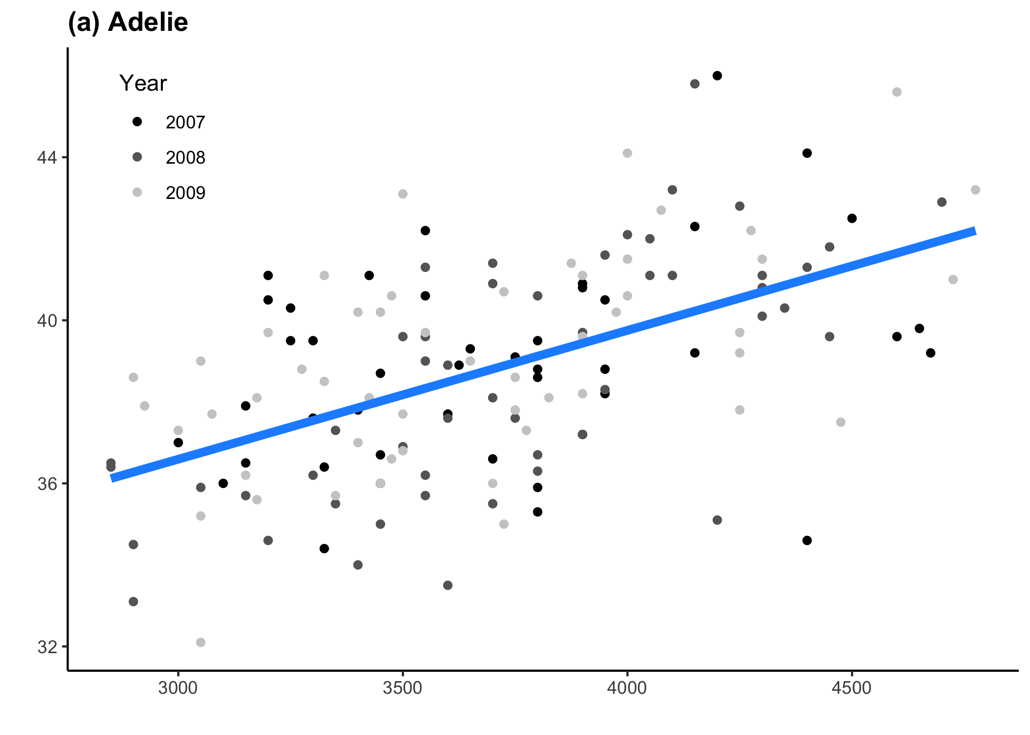
For each species, we’re going to generate scatterplots of bill length as a function of body mass, but we want to colour the points by year. We also want to fit a trend line, but we want the colour of each trend line to be different for species as well. ggplot2 will be unable to handle two separate colour grouping factors (i.e. species and year), so we’ll have to generate these individually.
In the end, let’s try to generate three plots stacked on top of each other. There are a couple of things we need to keep in mind (covered sequentially in the workshop, but not here).
- We only need an x axis title on the bottom plot and a y axis title in the middle plot.
- We only need a legend on one plot (not all)
- We need to separately specify the plot colours for the fit lines
- We need to separately specify the plot tag levels
# Again, we'll first specify an empty list outside the loop
plot_list <- list()
# Now, we'll go through the loop to generate the plots
for (penguin_sp in unique(penguins$species)) {
# This is where we'll specify the plot-specific details
if (penguin_sp == 'Adelie') {
x_axis_title <- '' # x axis title name
y_axis_title <- '' # y axis title name
legend_position <- c(0.1, 0.85) # legend position
penguin_colour <- 'dodgerblue' # colour of the trend line
penguin_tag <- '(a) Adelie' # plot tag level
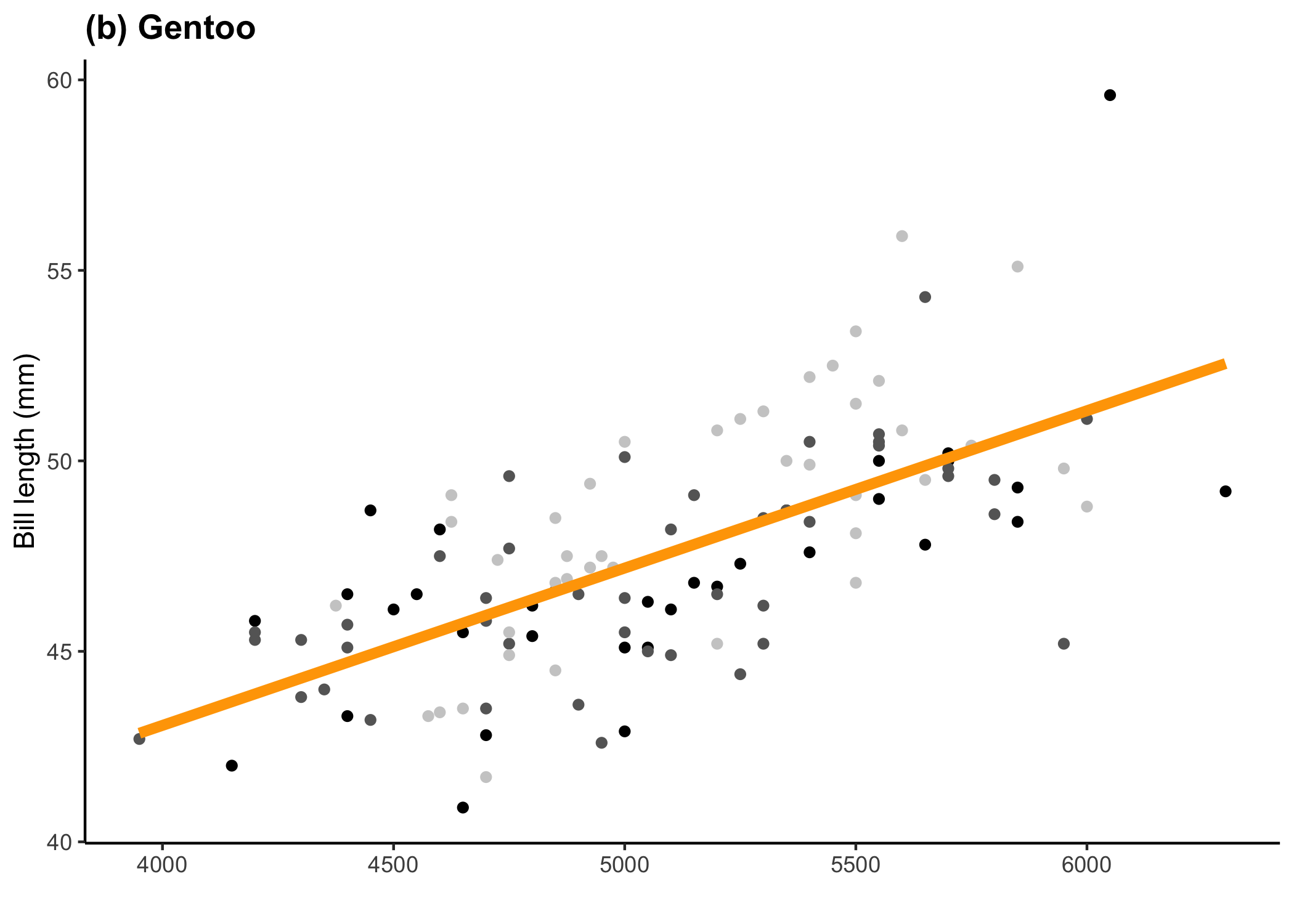
} else if (penguin_sp == 'Gentoo') {
x_axis_title <- ''
y_axis_title <- 'Bill length (mm)'
legend_position <- 'none'
penguin_colour <- 'orange'
penguin_tag <- '(b) Gentoo'
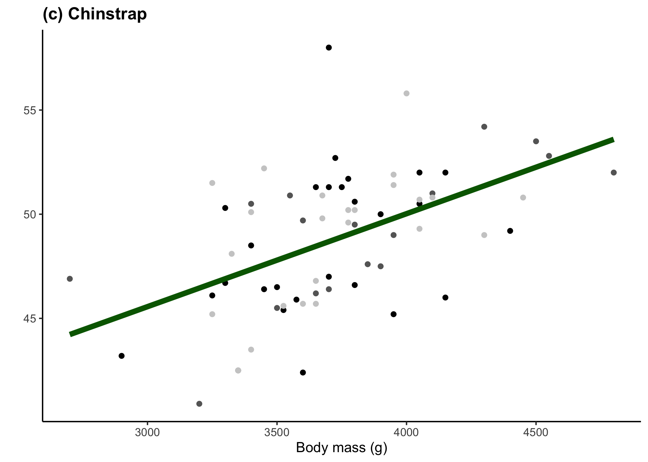
} else {
x_axis_title <- 'Body mass (g)'
y_axis_title <- ''
legend_position <- 'none'
penguin_colour <- 'darkgreen'
penguin_tag <- '(c) Chinstrap'
}
plot_list[[penguin_sp]] <-
penguins %>%
# First let's filter out the species we want
dplyr::filter(species == penguin_sp) %>%
# remove missing values
drop_na() %>%
# now let's generate the plot
ggplot(aes(x = body_mass_g, y = bill_length_mm)) +
# the points - convert year to a factor
geom_point(aes(colour = factor(year))) +
# the fitline - we'll just make it a straight line with no standard error
geom_smooth(colour = penguin_colour, linewidth = 2, se = FALSE,
method = 'lm', formula = 'y ~ x') +
# Specify the colours we want for year
scale_colour_manual(values = c('black', 'grey40', 'grey80')) +
# Add in the different titles
labs(x = x_axis_title,
y = y_axis_title,
colour = 'Year',
title = penguin_tag) +
# Specify a theme
theme_classic() +
theme(plot.title = element_text(face = 'bold', # make title bold
hjust = 0), # align text to the left
legend.position = legend_position)
}
plot_list[[1]]
plot_list[[2]]
plot_list[[3]]
Now we’ll bind all the plots together using patchwork
p <-
  plot_list[[1]] + plot_list[[2]] + plot_list[[3]] +
  plot_layout(ncol = 1)


p
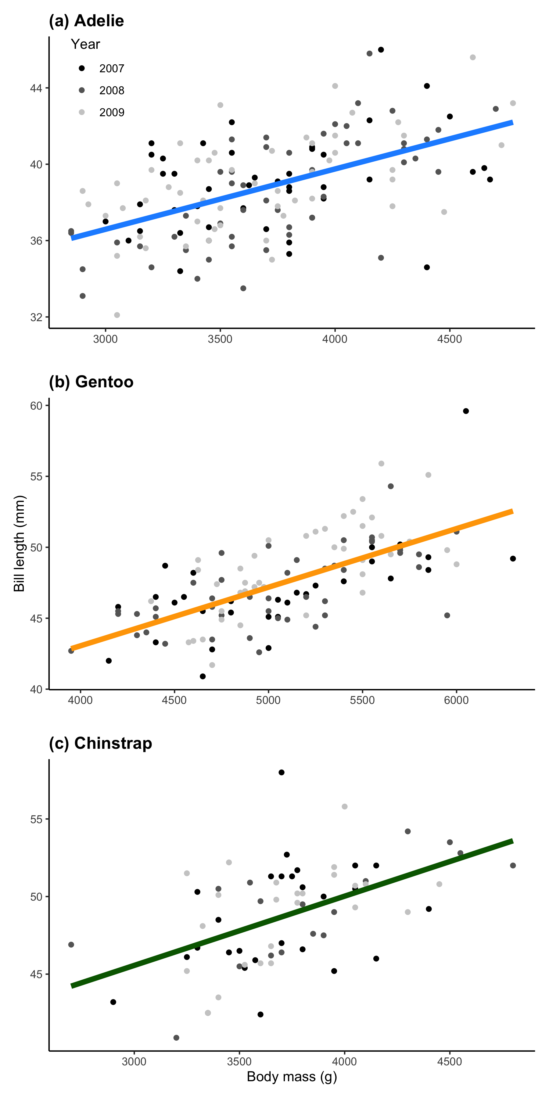
And there you go! The best part about generating individuals plots is that, when combined with patchwork, you can really customise how the plot will look. By controlling the relative sizes of all the plots, you can emphasise the importance of some over others (such as Fig. 3) or you can create overlapping plots with a negative plot_spacer() (such as Fig. 2).
Bootstrapping
The final use of for loops that we’re going to cover here is bootstrapping. Bootstrapping is the process by which you are resampling a dataset/model/etc. to create many simulated samples. For example, if you wanted to build a predictive model, you could use a cross-validation technique where you build your model on, say, 80% of your data and you predict its accuracy against the remaining 20%. Ideally, the first 80% of your data would have been chosen randomly. To assess the predictive accuracy, you could bootstrap this process multiple times and assess how good your model is at predicting. Similarly, a lot of machine learning algorithms these days (e.g. boosted regression trees) have a stochastic model-building process and can produce slightly different results based on the randomly chosen starting point. Therefore, these models are also typically bootstrapped across multiple iterations. Finally, people who are running simulations (such as the calculation of fish productivity), would bootstrap their simulations to assess how robust a set of outcomes is.
Here, we’re going to go with the first example and just run multiple linear models with a subset of the penguins dataset and predict on the remaining amount. Because this is not a workshop about linear modelling (check out our Everything you need to know about linear modelling workshop), we are just going to run a linear model of: $Bill~length \sim Body ~ mass$
So, the steps that we’re going to follow are:
- Randomly sample 80% of the dataset
- Build a model on the 80%
- Predict the bill length of the remaining 20%
- Model the predicted against the observed
- Extract the $r^2$ from each iteration
We are also going to include a progress bar so we can keep track of the progress of our bootstraps. This shouldn’t take too long with our data here, but some models take quite a while to run and this will be very helpful.
# First, we're going to generate a row number ID so we can easily separate the training set
# from the test set
penguins_data <-
  penguins %>%
  mutate(ID = row_number())

# This time, instead of creating an empty vector list, we'll create a dataframe with a column designating the bootstrap iteration and another with the perdicted R2 value
r2_data <-
  tibble(iteration = seq(1:1000),
         r2 = NA)

# Now to code the progress bar
pb <- txtProgressBar(min = 0, max = nrow(r2_data), style = 3)
## | | | 0%
# Ok, now let's run the for loop
for (i in 1:1000) {

  # Because we are randomly generating a portion of the data, we can set a seed at the beginning of
  # each iteration. That way, our results will be reproducible. Note: you don't want to generate a
  # single seed outside of the loop, because then all your values will be identical!
  set.seed(i)

  # First, we'll separate our data into a training set and a test set
  # The training set:
  data_train <-
    penguins_data %>%
    sample_frac(0.8)

  # The test set
  data_test <-
    anti_join(penguins_data, data_train, by = 'ID')

  # Now we'll create the model
  penguin_model <- lm(bill_length_mm ~ body_mass_g, data_train)

  # Create a new dataframe where we'll add the predictions to the original data
  data_predicted <-
    data_test %>%
    mutate(predicted_bill = stats::predict(penguin_model,
                                           newdata = tibble(body_mass_g = data_test$body_mass_g)))

  # Now, we'll run a model between our predicted and our observed values and extract the R2
  pred_mod <- lm(predicted_bill ~ bill_length_mm, data_predicted)

  # Finally, we'll infill the dataframe with the r2
  r2_data$r2[i] <- summary(pred_mod)$r.squared

  # Don't forget the progress bar!
  setTxtProgressBar(pb, i)

}
## | | | 1% | |= | 1% | |= | 2% | |== | 2% | |== | 3% | |== | 4% | |=== | 4% | |=== | 5% | |==== | 5% | |==== | 6% | |===== | 6% | |===== | 7% | |===== | 8% | |====== | 8% | |====== | 9% | |======= | 9% | |======= | 10% | |======= | 11% | |======== | 11% | |======== | 12% | |========= | 12% | |========= | 13% | |========= | 14% | |========== | 14% | |========== | 15% | |=========== | 15% | |=========== | 16% | |============ | 16% | |============ | 17% | |============ | 18% | |============= | 18% | |============= | 19% | |============== | 19% | |============== | 20% | |============== | 21% | |=============== | 21% | |=============== | 22% | |================ | 22% | |================ | 23% | |================ | 24% | |================= | 24% | |================= | 25% | |================== | 25% | |================== | 26% | |=================== | 26% | |=================== | 27% | |=================== | 28% | |==================== | 28% | |==================== | 29% | |===================== | 29% | |===================== | 30% | |===================== | 31% | |====================== | 31% | |====================== | 32% | |======================= | 32% | |======================= | 33% | |======================= | 34% | |======================== | 34% | |======================== | 35% | |========================= | 35% | |========================= | 36% | |========================== | 36% | |========================== | 37% | |========================== | 38% | |=========================== | 38% | |=========================== | 39% | |============================ | 39% | |============================ | 40% | |============================ | 41% | |============================= | 41% | |============================= | 42% | |============================== | 42% | |============================== | 43% | |============================== | 44% | |=============================== | 44% | |=============================== | 45% | |================================ | 45% | |================================ | 46% | |================================= | 46% | |================================= | 47% | |================================= | 48% | |================================== | 48% | |================================== | 49% | |=================================== | 49% | |=================================== | 50% | |=================================== | 51% | |==================================== | 51% | |==================================== | 52% | |===================================== | 52% | |===================================== | 53% | |===================================== | 54% | |====================================== | 54% | |====================================== | 55% | |======================================= | 55% | |======================================= | 56% | |======================================== | 56% | |======================================== | 57% | |======================================== | 58% | |========================================= | 58% | |========================================= | 59% | |========================================== | 59% | |========================================== | 60% | |========================================== | 61% | |=========================================== | 61% | |=========================================== | 62% | |============================================ | 62% | |============================================ | 63% | |============================================ | 64% | |============================================= | 64% | |============================================= | 65% | |============================================== | 65% | |============================================== | 66% | |=============================================== | 66% | |=============================================== | 67% | |=============================================== | 68% | |================================================ | 68% | |================================================ | 69% | |================================================= | 69% | |================================================= | 70% | |================================================= | 71% | |================================================== | 71% | |================================================== | 72% | |=================================================== | 72% | |=================================================== | 73% | |=================================================== | 74% | |==================================================== | 74% | |==================================================== | 75% | |===================================================== | 75% | |===================================================== | 76% | |====================================================== | 76% | |====================================================== | 77% | |====================================================== | 78% | |======================================================= | 78% | |======================================================= | 79% | |======================================================== | 79% | |======================================================== | 80% | |======================================================== | 81% | |========================================================= | 81% | |========================================================= | 82% | |========================================================== | 82% | |========================================================== | 83% | |========================================================== | 84% | |=========================================================== | 84% | |=========================================================== | 85% | |============================================================ | 85% | |============================================================ | 86% | |============================================================= | 86% | |============================================================= | 87% | |============================================================= | 88% | |============================================================== | 88% | |============================================================== | 89% | |=============================================================== | 89% | |=============================================================== | 90% | |=============================================================== | 91% | |================================================================ | 91% | |================================================================ | 92% | |================================================================= | 92% | |================================================================= | 93% | |================================================================= | 94% | |================================================================== | 94% | |================================================================== | 95% | |=================================================================== | 95% | |=================================================================== | 96% | |==================================================================== | 96% | |==================================================================== | 97% | |==================================================================== | 98% | |===================================================================== | 98% | |===================================================================== | 99% | |======================================================================| 99% | |======================================================================| 100%
close(pb) # it's good practice to close the progress bar
So now, if we look at the output r2_data, we can look at the
predictive accuracy of our model
ggplot(r2_data, aes(x = r2)) +
  geom_histogram(bins = 40)
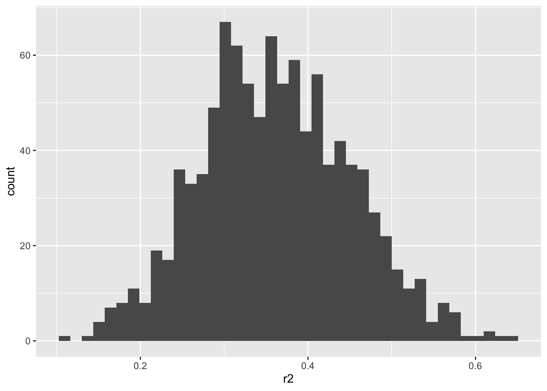
We have a $r^2$ of 0.36, which is not great for a predictive model…but not our problem for this example!
To keep this example simple, we only extracted the $r^2$ from this model, but obviously there are a bunch of other metrics/values that can come from this as well. A helpful tip, especially if your models take a while to run, when you’re first writing your code, don’t use the maximum number of bootstrapped iterations. You can usually find errors within 5-10 runs and that way, you’re not just sitting there waiting for your computer to finish running something incorrectly.
Nested for loops
In this final section, we’re going to go through a pretty simple nested for loop (i.e. a loop within a loop - loopception if you will). These can get pretty ugly pretty fast, so it’s best to break things down into small tasks and troubleshoot as you code.
Let’s say, we want the minimum and maximum flipper length again for each species of penguin, for each year that they were sampled. The key here is that every species was sampled in each year - if you have gaps, then you would need to introduce if next or if break statements. Remember when we would specify empty lists and empty dataframes outside the loop? Well, when you’re nesting, you basically do the same thing - we can designate objects inside the first loop but outside the second. Tip: make sure you keep track of what your iterating object is for each loop - mixing up i with j can really mess things up.
# We'll designate an empty list to infill with species-level data
species_list <- list()

# Now we'll run the loops. The outter loop is the species-level loop.
# The inner loop is the year-level loop
for (i in unique(penguins$species)) {

  # First, we'll subset the data at the species level
  species_subset <-
    penguins %>%
    dplyr::filter(species == i)

  # We will also specify a separate list to infill with year-specific data
  year_list <- list()

  # now we'll run the year-specific loop
  for (j in unique(penguins$year)) {

    # Now we'll subset the species_subset dataframe by year
    year_subset <-
      species_subset %>% # take the dataframe from the species loop
      dplyr::filter(year == j)

    # Now we can specify the dataframe into the empty datalist above
    year_list[[j]] <-
      rbind(year_subset %>%
              dplyr::slice_min(bill_length_mm), # take the minimum
            year_subset %>%
              dplyr::slice_max(bill_length_mm)) # take the maximum
  }

  # Now, we'll bind together the year-level dataframes into our empty list that
  # we set outside
  species_list[[i]] <-
    do.call(rbind, year_list)

  # Let's leave a nice message for ourselves
  cat(paste('Finishing species:', i, '\n', sep = ' '))

}
## Finishing species: Adelie
## Finishing species: Gentoo
## Finishing species: Chinstrap
species_list[[1]]
| species | island | bill_length_mm | bill_depth_mm | flipper_length_mm | body_mass_g | sex | year |
|---|---|---|---|---|---|---|---|
| Adelie | Torgersen | 34.1 | 18.1 | 193 | 3475 | NA | 2007 |
| Adelie | Torgersen | 46.0 | 21.5 | 194 | 4200 | male | 2007 |
| Adelie | Dream | 33.1 | 16.1 | 178 | 2900 | female | 2008 |
| Adelie | Torgersen | 45.8 | 18.9 | 197 | 4150 | male | 2008 |
| Adelie | Dream | 32.1 | 15.5 | 188 | 3050 | female | 2009 |
| Adelie | Biscoe | 45.6 | 20.3 | 191 | 4600 | male | 2009 |
species_list[[2]]
| species | island | bill_length_mm | bill_depth_mm | flipper_length_mm | body_mass_g | sex | year |
|---|---|---|---|---|---|---|---|
| Gentoo | Biscoe | 40.9 | 13.7 | 214 | 4650 | female | 2007 |
| Gentoo | Biscoe | 59.6 | 17.0 | 230 | 6050 | male | 2007 |
| Gentoo | Biscoe | 42.6 | 13.7 | 213 | 4950 | female | 2008 |
| Gentoo | Biscoe | 54.3 | 15.7 | 231 | 5650 | male | 2008 |
| Gentoo | Biscoe | 41.7 | 14.7 | 210 | 4700 | female | 2009 |
| Gentoo | Biscoe | 55.9 | 17.0 | 228 | 5600 | male | 2009 |
species_list[[3]]
| species | island | bill_length_mm | bill_depth_mm | flipper_length_mm | body_mass_g | sex | year |
|---|---|---|---|---|---|---|---|
| Chinstrap | Dream | 42.4 | 17.3 | 181 | 3600 | female | 2007 |
| Chinstrap | Dream | 58.0 | 17.8 | 181 | 3700 | female | 2007 |
| Chinstrap | Dream | 40.9 | 16.6 | 187 | 3200 | female | 2008 |
| Chinstrap | Dream | 54.2 | 20.8 | 201 | 4300 | male | 2008 |
| Chinstrap | Dream | 42.5 | 17.3 | 187 | 3350 | female | 2009 |
| Chinstrap | Dream | 55.8 | 19.8 | 207 | 4000 | male | 2009 |
And now, we can bind them all together into a single dataframe
penguins_year <-
  do.call(rbind, species_list)

penguins_year
| species | island | bill_length_mm | bill_depth_mm | flipper_length_mm | body_mass_g | sex | year |
|---|---|---|---|---|---|---|---|
| Adelie | Torgersen | 34.1 | 18.1 | 193 | 3475 | NA | 2007 |
| Adelie | Torgersen | 46.0 | 21.5 | 194 | 4200 | male | 2007 |
| Adelie | Dream | 33.1 | 16.1 | 178 | 2900 | female | 2008 |
| Adelie | Torgersen | 45.8 | 18.9 | 197 | 4150 | male | 2008 |
| Adelie | Dream | 32.1 | 15.5 | 188 | 3050 | female | 2009 |
| Adelie | Biscoe | 45.6 | 20.3 | 191 | 4600 | male | 2009 |
| Gentoo | Biscoe | 40.9 | 13.7 | 214 | 4650 | female | 2007 |
| Gentoo | Biscoe | 59.6 | 17.0 | 230 | 6050 | male | 2007 |
| Gentoo | Biscoe | 42.6 | 13.7 | 213 | 4950 | female | 2008 |
| Gentoo | Biscoe | 54.3 | 15.7 | 231 | 5650 | male | 2008 |
| Gentoo | Biscoe | 41.7 | 14.7 | 210 | 4700 | female | 2009 |
| Gentoo | Biscoe | 55.9 | 17.0 | 228 | 5600 | male | 2009 |
| Chinstrap | Dream | 42.4 | 17.3 | 181 | 3600 | female | 2007 |
| Chinstrap | Dream | 58.0 | 17.8 | 181 | 3700 | female | 2007 |
| Chinstrap | Dream | 40.9 | 16.6 | 187 | 3200 | female | 2008 |
| Chinstrap | Dream | 54.2 | 20.8 | 201 | 4300 | male | 2008 |
| Chinstrap | Dream | 42.5 | 17.3 | 187 | 3350 | female | 2009 |
| Chinstrap | Dream | 55.8 | 19.8 | 207 | 4000 | male | 2009 |
Congratualtions! You have now gone through and learned how to implement for loops in R! Obviously, there are so many other places where you can use for loops, but hopefully this tutorial was helpful in providing you with a baseline understanding and some common implementation techniques!