The significance of p-values
(and no we’re not just preaching Bayesian)
What are p-values? Why do we use them? Why are people getting sooo bent out of shape about using them? Do we need to use them? If I don’t want to use p-values, do I have to do Bayesian? These are all great questions that we’ll address in this tutorial/guide. Despite the name of our blog, the purpose of this tutorial isn’t to convert everyone to Bayesian (although we provide pretty good reason to do so). Instead, we want ecologists to understand the use of p-values, its shortcomings, and how to better-interpret your model results in a meaningful way.
In this tutorial, we will uncover the basics of p-values/significance testing, why we used to rely on them, and how we can move forward with the interpretation of our models. We won’t dive deep into model interpretation; check-out our Model Interpretation tutorial, which is coming soon. By the end of this tutorial, you will be able to:
- Understand the basics of p-values and why we use them (without too much math)
- Move forward beyond simply relying on p-values to infer effects
- Get a baseline understanding of the difference between frequentist and Bayesian statistics ;)
Part 1: The basics of p-values
What are p-values? Technically, a p-value is the probability of obtaining the results that you have observed given that the null hypothesis is true. In layman’s terms, you can think of this as the probability of getting the results you’ve observed due to chance alone. So, if p=0.95, we can say that there is a 95% chance that our results are due to chance. In stats terms, we would say that the effect is non-significant and we cannot reject the null hypothesis.
In biological systems, typically our null hypothesis is no effect. For example, if we wanted to know the effect of temperature on the growth of fish, our null hypothesis would be that there is no effect of temperatrue on growth. Simple, right? Unfortunately not.
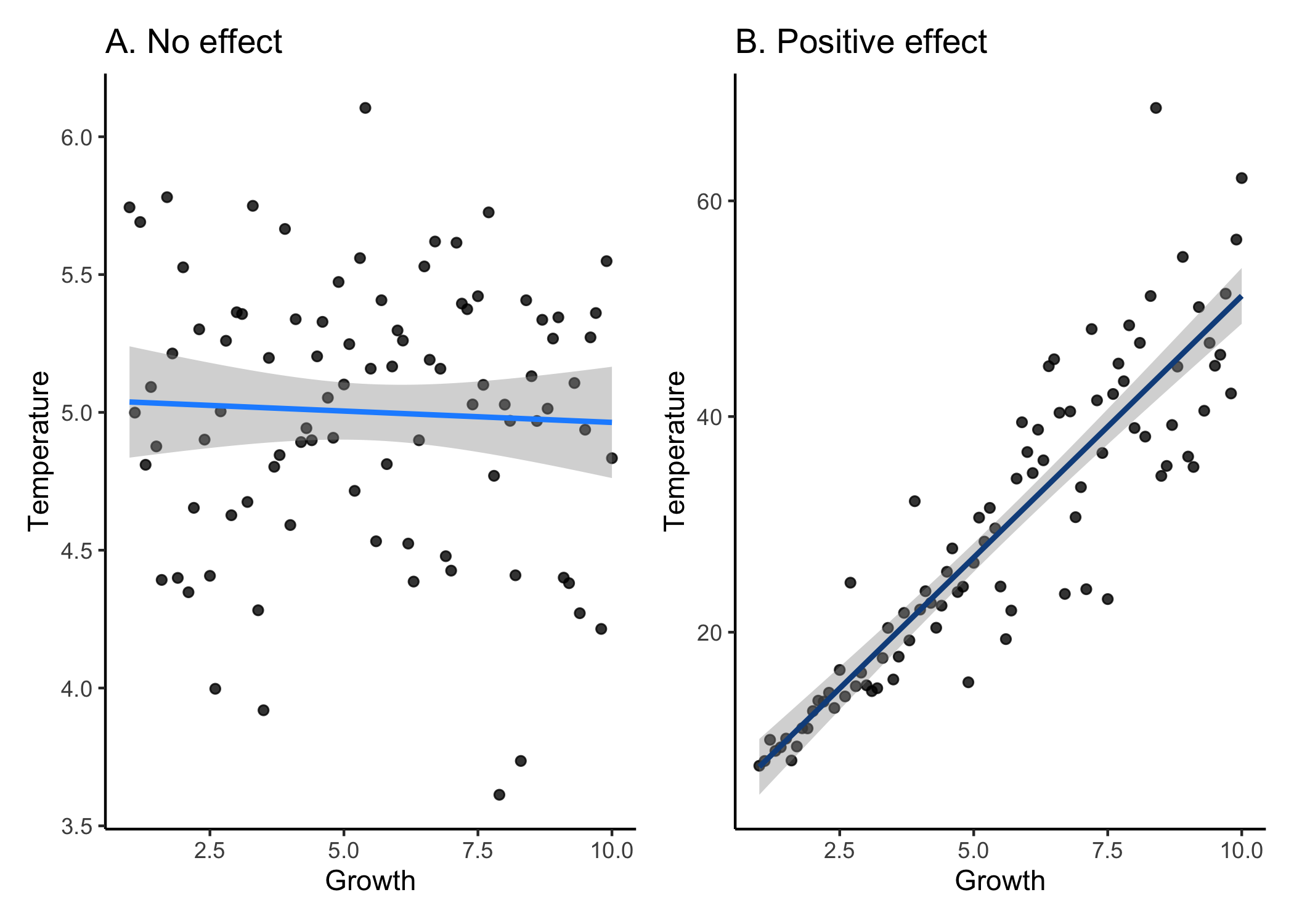
So let’s take a quick step back. P-values are continuous between 0 and 1, so stats people tell us that we need a cut-off value for which we can say whether or not we are rejecting the null hypothesis. This value is known as an alpha value, which we decide. Who’s we? Well, the general world of ecologists have all accepted an alpha value of 0.05. Why 0.05? That’s an excellent question. You would think this would arise from an extensive survey and discussion among scientists all over the world. But of course this isn’t what happened. Realistically, some dude named sir Henry of Alpha in the early 1900s who had to calculate p-values by hand probably chose 0.05 because that was the width of their quill. Or the thickness of their scroll. Or the amount of ankle they were allowed to show. Is this actually the reason why we use 0.05? Probably not. But is the real reason any less arbitrary? Definitely not.
So if p>0.05, we have accepted that this means that the effect is non-significant and we can’t reject the null hypothesis. If p<0.05, then the effect is significant and we reject the null. That’s all fine and dandy, but does that really make sense? If we think back to the definition of a p-value, it’s the probability of getting your results given that the null hypothesis is true. So, if p=0.051 then the effect is non-significant; but, if p=0.049, then the effect is significant. In ecology, we have gotten into the habit of applying a binary yes/no designation to a continuous scale of probabilities. Biologically speaking, is there really a difference between 5.1% versus 4.9%? Realistically, there probably isn’t a difference. Still don’t believe me that this is arbitrary? Well, in other fields, they use a different alpha level to designate significance. One that they decided was ok. Let that sink in.
Finally, you can’t really calculate p-values for all analyses. For example, the package lme4 recently got rid of their p-values in the model outputs because they cannot accurately be calculated…so now what?
Part 2: Effect sizes
When we had to rely on tables to do calculations, sure it’s easier to just accept that there is an effect at a certain cut-off value. Now, given the massive increase in computing power and the extensive use of stats in ecology, we can do better. Introducing: effect sizes.
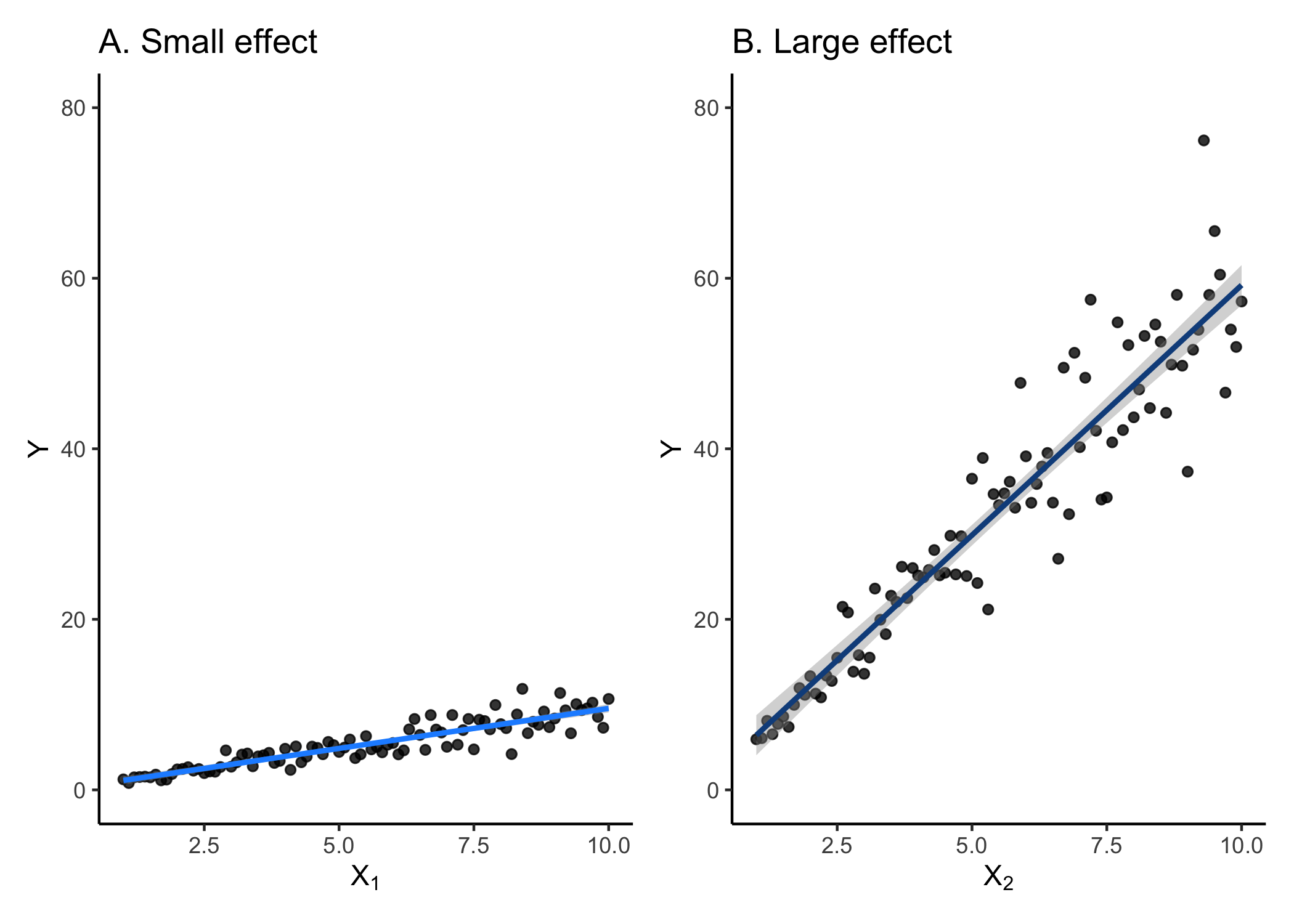
Effect sizes indicate the magnitude of the effect of an independent variable. Instead of just saying that a variable has a significant effect, we can infer whether or not it has a large effect of small effect.
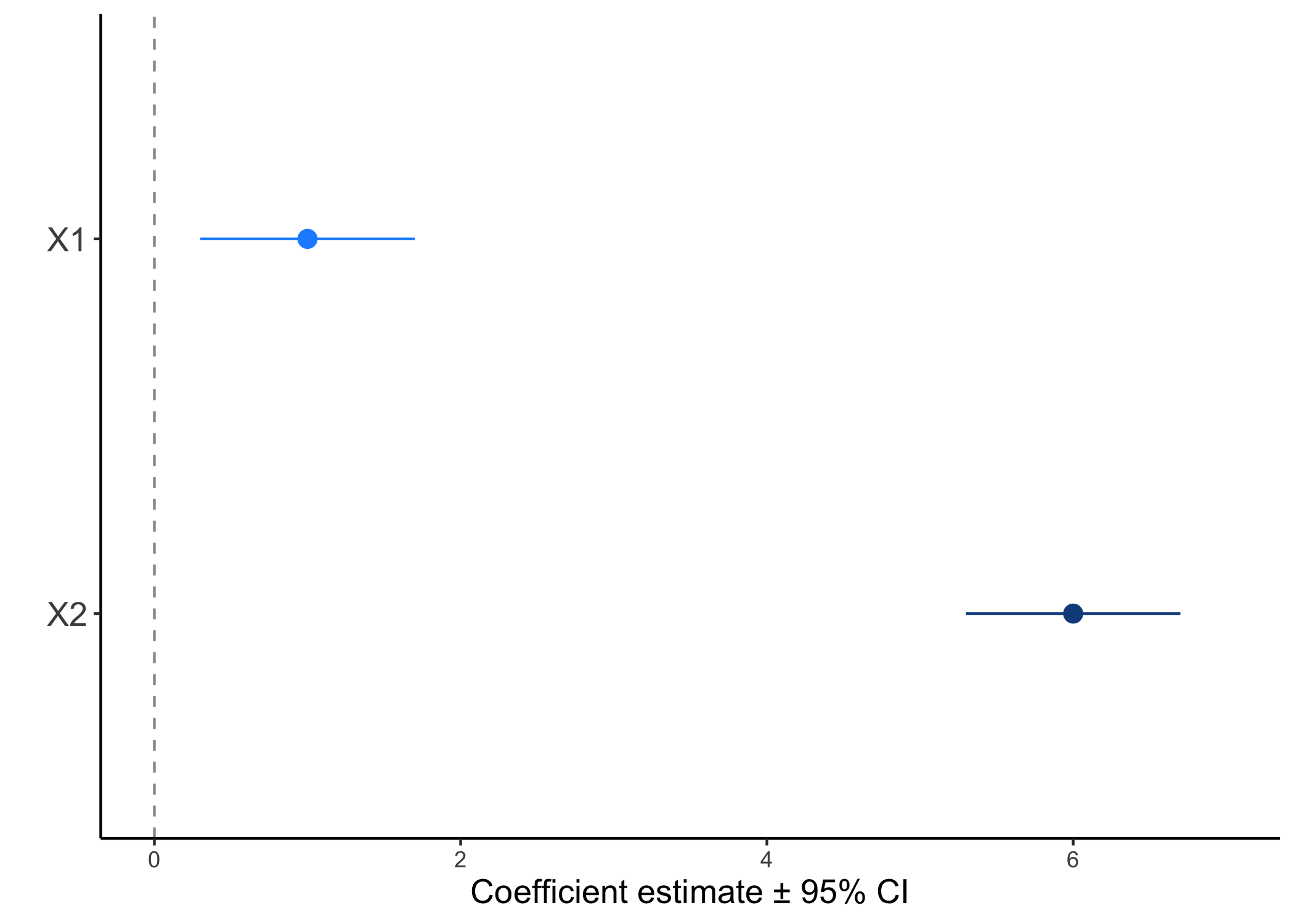
This plot is known as a coefficient plot and is one way of directly denoting effect sizes. The coefficients plotted are just the slope estimates from your model and are shown with 95% confidence intervals (CI). In frequentist statistics, the confidence interval can be described as: “If we take a bunch of repeated samples from the same population and calculate a new CI each time, the culmulation of CIs will bracket the true population value 95% of the time”. It’s rather complex, but for the sake of argument it’s just a way to show uncertainty around an estimate.
In this example, we have two continuous variables X1 and X2. In both cases, they would have significant effects. Biologically speaking though, does that mean they have the same effect? We can see that X1 has a smaller effect than X2, or the slope between y ~ X2 is steeper than that of y ~ X1. Of course this can be conflated by whatever units your x variables are in (what if X1 ranged from 0.1-0.5 and X2 ranged from 100-500). This is one of the reasons why it’s a good rule of thumb to scale and center you independent variables - that way, you can use coefficient estimates to compare relative effect sizes.
There are a number of different ways to measure effect sizes. The following examples are more common for meta-analyses and less common for simply interpreting your models. One way is to use Pearson’s r correlation. If you recall, correlation measures how tight the relationship between two variables is. It varies from -1 (perfect negative fit) and 1 (perfect positive fit). We would say that the effect is small if the correlation is low (~0.1) and large if the correlation is high (>0.5).
Another common effect size measurement is Cohen’s d. Cohen’s d is typically used to compare the means between two groups from one population (e.g., control vs. treatment). For this reason, it’s most commonly used in meta-analyses. It renders the comparison of two groups down to standard deviation units and can thus be easily compared across studies.
To get a quick taste of other types of effect sizes, click here.
Part 3: B-B-B-BAYESIAN!
A super-rapid brief intro

Ok, so now that we know that we don’t need p-values, we’re basically one step closer to Bayesian statistics. At the most basic level, Bayesian and frequentist statistics differ in their definitions of probability. In frequentist, probability is defined of the proportion of times an event would occur if we repeated a random trial over and over again under the same conditions (e.g., if we toss a fair coin, what is the probability of 10 heads in a row). Conversely, the Bayesian definition of probability is expressed as the degree of belief in an event (e.g., what is the probability that hippos are the sister group to the whales?).
Because Bayesian and Frequentist differ in their definitions of probability, we don’t report the results in the same way. Although the interpretation of the coefficient estimates are essentially identical (unless you use priors), we report uncertainty slightly differently. Recall that we use confidence intervals in frequentist statistics to propagate uncertainty (definition above in Part 2). In Bayesian stats, we use credible intervals, which are defined as there being a X% chance that the true population lies within this range. It’s ok to use a 95% credible interval, but this is actually a point of contention and Richard McElreath goes into detail about how this is as arbritary of a choice as p=0.05 in his book Statistical Rethinking.
We won’t bog down too much into what defines Bayesian statistics (it will have its own tutorial, also coming soon). For the purpose of this tutorial/rant, the take-home message is that because frequentist and Bayesian statistics differ in their use of probabilities, you don’t use p-values in Bayesian stats. Although you can use something called Bayes’ factor, which simply compares models to one-another and doesn’t necessarily test a null hypothesis, we rely on interpreting our models using effect sizes and the uncertainty around these estimates.
Some final thoughts
Here, we’ve provided you with a relatively short rant as to why we, as ecologists, should start to deviate away from solely using p-values. Of course, this doesn’t mean that we have to ditch them altogether, but instead let’s not rely on them as the only way to report results. Reporting effect sizes not only gets around the fact that p=0.05 is a ridiculous cut-off (especially if p is only slightly higher than 0.05), but it also shows the magnitude of an effect. As biologists, this is what is truly interesting! We know that temperature affects metabolic rate, but by how much?
Unfortunately, because our field is still filled with a lot of…traditional scientists who were taught step-wise regression and ANOVAs, you might face some resistance from reviewers if you try to publish without p-values. The war against p-values is definitely growing and we have no doubt that it’ll soon be the norm to ignore them.