Interpreting Models with Interactions
One of the most common questions that comes up in stats help discussions is “how do I interpret my interaction term?” (or its cousin “why are my main effects not significant anymore when I add an interaction?”). And I think the reason it comes up so often, despite interactions being a pretty straightforward and common component of linear models, is that there isn’t a super clean answer. My default response is to tell people to draw out the model output for each combination of variables they have, and I’m usually met with a “but what does the coefficient mean?” because people want a one line answer. Tragically, that simple answer won’t make sense until you have a deeper understanding of what is going on in your model, so we’re going to get into that here. In this tutorial we’ll cover:
Part 1
- Why adding an interaction term changes your main effects so much
- What main effects actually represent with and without an interaction
- How centering data can help reduce confusion in interpreting continuous variables
Part 2
- What the interaction term actually represents
- How to mentally visualize your model output before you even plot anything
Part 1: Rethinking Main Effects
a.k.a. Your coefficient plots aren’t as helpful as you think they are
I first ran into issues interpreting interactions during my Honours project on lizards, so we’ll use a lizard example here (because everything is better with lizards)! We’ll make up some data so they’re a little cleaner and we know the true patterns underlying them.
Let’s say we have 100 lizards, 50 male and 50 female, and we’re interested in their home range size. Given our expertise on lizards, we have reason to believe that sex and body size may play a role in determining home range size. We are their god in this hypothetical situation, so we actually KNOW that they do; let’s say male lizards have a larger home range than females, and home range size increases with lizard body size in males, but stays constant in females. We can generate some data to match these patterns:
#generate sequence of body sizes for each sex
males <- tibble(body_size = seq(from = 4, to = 8, length.out = 50))
females <- tibble(body_size = seq(from = 4, to = 8, length.out = 50))

#set seed for reproducibility
set.seed(123)

#for females, home range will be constant with body size, with a little bit of
#error around the mean
females <- females %>%
  mutate(home_range = rnorm(50, mean = 5, sd = 0.5),
         sex = factor("female"))

#for males, home range will increase with body size (by 1m^2 per cm body
#length), with a little bit of error around the mean
males <- males %>%
  mutate(home_range = rnorm(50, mean = 1, sd = 0.1)*body_size + 2,
         sex = factor("male"))

#now put the males and females together
df <- bind_rows(females, males)
Let’s briefly look at this data to see if we notice any obvious patterns.
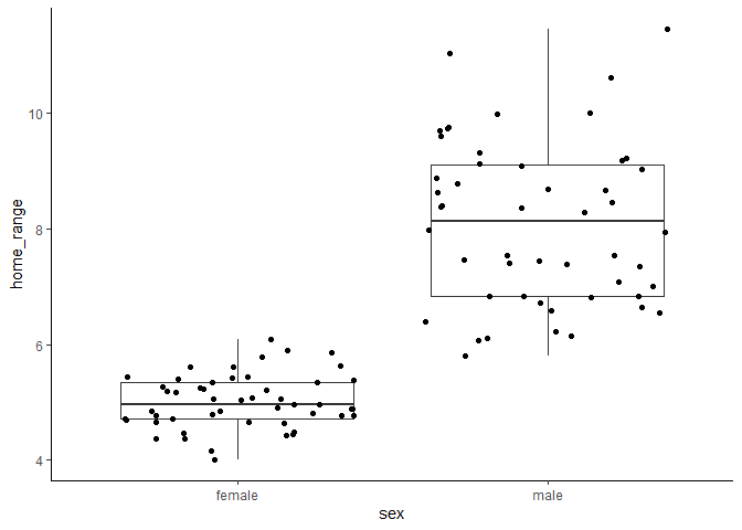
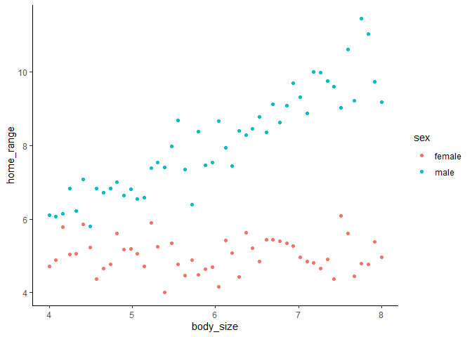
Here we can see that males clearly have larger home range sizes than females, and that their home ranges increase with increasing body size, while females’ do not. This should be really clear in the model, right? If we run a model without an interaction, here’s what we see.
mod1 <- lm(home_range ~ sex + body_size, data = df)
summary(mod1)
##
## Call:
## lm(formula = home_range ~ sex + body_size, data = df)
##
## Residuals:
##      Min       1Q   Median       3Q      Max
## -1.55281 -0.61341 -0.02224  0.55708  2.40467
##
## Coefficients:
##             Estimate Std. Error t value Pr(>|t|)
## (Intercept)  1.78567    0.44004   4.058    1e-04 ***
## sexmale      3.08425    0.16650  18.525  < 2e-16 ***
## body_size    0.53859    0.07067   7.621 1.69e-11 ***
## ---
## Signif. codes:  0 '***' 0.001 '**' 0.01 '*' 0.05 '.' 0.1 ' ' 1
##
## Residual standard error: 0.8325 on 97 degrees of freedom
## Multiple R-squared:  0.8053, Adjusted R-squared:  0.8013
## F-statistic: 200.6 on 2 and 97 DF,  p-value: < 2.2e-16
This model output tell us that males, on average across body sizes, have a home range that is 3.1 m2 larger than females, and that averaged across sexes, we expect a 0.54 m2 increase in home range size with every cm increase in body size. (Note that the slope we used for females was 0 and the slope we used for males is 1, and since we had equal numbers of males and females, it makes sense that our averaged slope is halfway between the two).
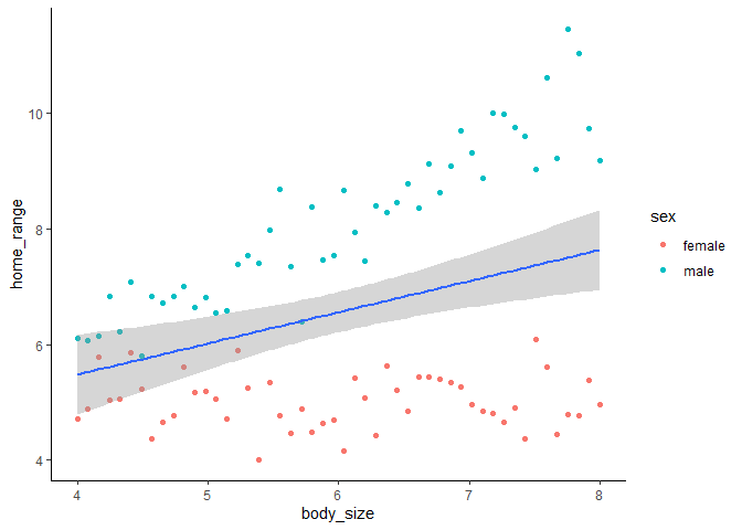
Now let’s add an interaction into the model, since, as the lizard god, we know that the effect of body size on home range size should be different for males and females.
mod2 <- lm(home_range ~ sex * body_size, data = df)
summary(mod2)
##
## Call:
## lm(formula = home_range ~ sex * body_size, data = df)
##
## Residuals:
##      Min       1Q   Median       3Q      Max
## -1.39655 -0.33420 -0.00423  0.33036  1.44480
##
## Coefficients:
##                    Estimate Std. Error t value Pr(>|t|)
## (Intercept)        5.067085   0.379911  13.338  < 2e-16 ***
## sexmale           -3.478568   0.537276  -6.474 4.03e-09 ***
## body_size         -0.008314   0.062132  -0.134    0.894
## sexmale:body_size  1.093804   0.087868  12.448  < 2e-16 ***
## ---
## Signif. codes:  0 '***' 0.001 '**' 0.01 '*' 0.05 '.' 0.1 ' ' 1
##
## Residual standard error: 0.5176 on 96 degrees of freedom
## Multiple R-squared:  0.9255, Adjusted R-squared:  0.9232
## F-statistic: 397.7 on 3 and 96 DF,  p-value: < 2.2e-16
Here’s where things get interesting. Even though we know males have larger home ranges, our model suggests that they actually have way smaller ones (by about 3.5 m2). It also suggests that there is a tiny negative effect of body size (although this isn’t significant). What’s going on?
Well, the moment you add an interaction to a model you completely change the meaning of what main effects actually are!
In the first case, without an interaction, the coefficient for each main effect represents the effect of a variable averaged across all levels (or values) of the other variable(s). When you add an interaction, the coefficient for each main effect represents the effect of a variable at the intercept levels of the other variable(s).
In the case of our model, the intercept values are for females with a body size of zero cm. This means our body size main effect term is only for females and the sex effect is only for individuals with a body size of 0. Note that if you are unsure of what the intercept values are for your data, they will always be 0 for continuous variables and the first level of categorical variables which you can check with:
#note that variable must be a factor, not a character to use levels()
levels(df$sex)
## [1] "female" "male"
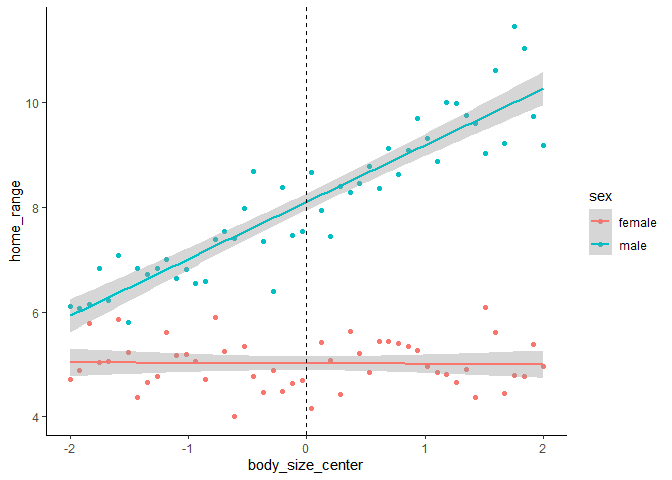
To visualize what this means, let’s extend the x axis of our previous figure.
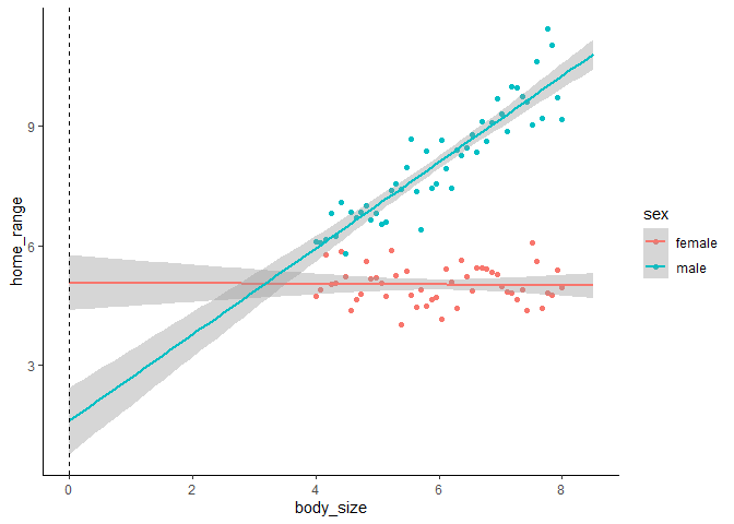
The dotted line shows us where our model coefficients are being drawn from. The intercept is where the pink line (for females) crosses the dotted line, the effect of sex (for males) is the difference between where the pink line and blue line cross the dotted line, the effect of body size is the slope of the pink line, and the interaction is the difference between the slopes of the blue and pink lines. Now our model output makes a little more sense, but it’s kind of annoying to have to mentally extrapolate beyond the range of our data to interpret our model coefficients.
Thankfully, there is a very easy fix to this confusing problem. If you have multiple continuous variables with different units of measurement in your model, it’s generally good practice to standardize (i.e. center and divide by their standard deviation) them. This allows you to compare relative effects of different variables. For instance, if you had one variable measured in cm with an effect size of 0.2 and you converted it to m, the effect size would grow to 20! (This is because a 1 unit change in metres would correspond to a 100 unit change in cm). We can standardize variables very easily in R with the scale() function. You can apply this either to a data frame
df <- df %>% mutate(body_size_stand = scale(body_size))
or within the model itself.
lm(home_range ~ scale(body_size) + sex, data = df)
Let’s see how this changes our coefficients:
df <- df %>%
  mutate(body_size_stand = scale(body_size))
mod_stand <- lm(home_range ~ sex * body_size_stand, data = df)
summary(mod_stand)
##
## Call:
## lm(formula = home_range ~ sex * body_size_stand, data = df)
##
## Residuals:
##      Min       1Q   Median       3Q      Max
## -1.39655 -0.33420 -0.00423  0.33036  1.44480
##
## Coefficients:
##                          Estimate Std. Error t value Pr(>|t|)
## (Intercept)              5.017202   0.073194  68.547   <2e-16 ***
## sexmale                  3.084254   0.103512  29.796   <2e-16 ***
## body_size_stand         -0.009843   0.073562  -0.134    0.894
## sexmale:body_size_stand  1.295025   0.104033  12.448   <2e-16 ***
## ---
## Signif. codes:  0 '***' 0.001 '**' 0.01 '*' 0.05 '.' 0.1 ' ' 1
##
## Residual standard error: 0.5176 on 96 degrees of freedom
## Multiple R-squared:  0.9255, Adjusted R-squared:  0.9232
## F-statistic: 397.7 on 3 and 96 DF,  p-value: < 2.2e-16
We can see that the effect of body size is still ~0 because it is still based on females only (since we didn’t standardize our categorical variable), but our main effect of sex now makes more biological sense based on how we generated the data. We can plot it below.

Our new intercept now lies at the mean body size, rather than at 0cm. So our model with an interaction is still representing the effect of a variable at the intercept levels of the other variable(s), we just changed what the intercept values are to help us with our interpretation. Note that when we’re describing the effect sizes, each unit in this case is 1 SD (of the range of body sizes in this population) rather than 1cm.
Having our effect sizes listed in actual units (e.g. body size in cm) may be beneficial in some cases when you want to be able to make statements such as “for every cm increase in body size, we would expect to see an X increase in home range size). In this case, we don’t necessarily want to divide by the SD of variable, but we can still center using scale(). scale() has two arguments, center and scale, which by default are both set to true. If we use scale(scale = FALSE), we can now simply center our data around the mean value of the continuous variable(s).
df <- df %>%
  mutate(body_size_center = scale(body_size, scale = FALSE))
mod_center <- lm(home_range ~ sex * body_size_center, data = df)
summary(mod_center)
##
## Call:
## lm(formula = home_range ~ sex * body_size_center, data = df)
##
## Residuals:
##      Min       1Q   Median       3Q      Max
## -1.39655 -0.33420 -0.00423  0.33036  1.44480
##
## Coefficients:
##                           Estimate Std. Error t value Pr(>|t|)
## (Intercept)               5.017202   0.073194  68.547   <2e-16 ***
## sexmale                   3.084254   0.103512  29.796   <2e-16 ***
## body_size_center         -0.008314   0.062132  -0.134    0.894
## sexmale:body_size_center  1.093804   0.087868  12.448   <2e-16 ***
## ---
## Signif. codes:  0 '***' 0.001 '**' 0.01 '*' 0.05 '.' 0.1 ' ' 1
##
## Residual standard error: 0.5176 on 96 degrees of freedom
## Multiple R-squared:  0.9255, Adjusted R-squared:  0.9232
## F-statistic: 397.7 on 3 and 96 DF,  p-value: < 2.2e-16
Now our effects are represented in units of the continuous variable rather than in SD.
Part 2: What the hell does the interaction coefficient actually mean?
a.k.a. y = mx + b-ing this shit
Ok sweet, we now have a pretty good idea how to interpret main effects. The next step is to interpret the interaction term. Exactly how to interpret an interaction term is going to depend on whether the variables are categorical, continous, or a mix of both. Again, everyone wants an easy answer here and hates it when I tell them to write it out but TOO BAD, that’s what we’re going to do. Once you get the hang of it, you’ll be able to interpret it pretty quickly in your head, but the only way to really get it is to use our old friend y = mx + b. There are some great packages in R that can help visualize these interactions (e.g. emmeans), but it is super helpful to know how to interpret them yourself before relying on a package to deal with it under the hood!
All linear models are just y = mx + b with some fancy variations. When in doubt, always start by writing your y = mx + b statement out.
- y is your dependent variable
- x is your independent variable(s)
- m is your model coefficient(s)
- b is your intercept
You can have multiple m’s and x’s, which we’ll denote as m1, m2, etc. and x1, x2, etc.
“Now Hannah,” you might be thinking, “there isn’t any interaction term in y = mx + b”. Well this is just one of those fancy variations I was talking about. The interaction coefficient in a linear model is still an “m” term in our equation, but instead of using it on a single variable (e.g. m1*x1), we use it on two (e.g. m1,2*x1*x2). Let’s see how this plays out for different types of variables.
One categorical and one continuous variable
Let’s go back to our lizard problem as an example again. We have one categorical variable in our model (sex, with female as the intercept level and male as the next level) and one continuous variable (body size, measured in cm - we’ll use the centered version from above). In y = mx + b form, our model looks like:
home_range = msex * sexmale + mbody_size * body_size_center + minteraction * sexmale*body_size_center + intercept
And our model output looks like this:
summary(mod_center)
##
## Call:
## lm(formula = home_range ~ sex * body_size_center, data = df)
##
## Residuals:
##      Min       1Q   Median       3Q      Max
## -1.39655 -0.33420 -0.00423  0.33036  1.44480
##
## Coefficients:
##                           Estimate Std. Error t value Pr(>|t|)
## (Intercept)               5.017202   0.073194  68.547   <2e-16 ***
## sexmale                   3.084254   0.103512  29.796   <2e-16 ***
## body_size_center         -0.008314   0.062132  -0.134    0.894
## sexmale:body_size_center  1.093804   0.087868  12.448   <2e-16 ***
## ---
## Signif. codes:  0 '***' 0.001 '**' 0.01 '*' 0.05 '.' 0.1 ' ' 1
##
## Residual standard error: 0.5176 on 96 degrees of freedom
## Multiple R-squared:  0.9255, Adjusted R-squared:  0.9232
## F-statistic: 397.7 on 3 and 96 DF,  p-value: < 2.2e-16
We can plug in these coeffcients into our written model:
home_range = 3.08 * sexmale - 0.008 *body_size_center + 1.09 *sexmale*body_size_center + 5.02
Remember, our “intercept lizard” is a female lizard with the mean body size (since we’ve centered our data). We can see that by plugging our hypothetical lizard into our model.
- Term 1 (msex *sexmale) would be 0, because sex is a dummy variable in this case and coded as 0s and 1s. So for sexmale, male would be treated as a 1 and female as a 0 since it is the first level of this factor. 3.08 * 0 is 0, so this term drops out when we have a female lizard.
- Term 2 (mbody_size *body_size_center) would also be 0 because our body size variable is centered. Since we subtract the mean body size from each of the observations, a lizard at the mean body size would have a centered body size of 0. -0.008 * 0 is 0, so this term drops out.
- Term 3 (minteraction *sexmale*body_size_center) also drops out since we know that sex and body size would both be set to 0.
This leaves us with just the intercept, meaning that term alone tells us the home range size of a female lizard of mean body size. We can then use this breakdown to understand what our model says about lizards without these “intercept characteristics”.
-
For any female lizards, the sex term and the interaction term will always be dropped because females are coded as the base level for this factor; if we set sexmale to zero, these terms both become 0. This means that the home range size can just be calculated for females as:
home_range = mbody_size*body_size_center + intercept
-
For male lizards, our interaction term now affects the slope of the body size term. For male lizards, we plug in a 1 for the sexmale variable in Terms 1 and 3. This means our equation reduces to home_range = msex + mbody_size*body_size_center + minteraction*body_size_center + intercept (since 1*x is equal to x). This can be further reduced by combining terms 2 and 3; you’ll remember from high school math that a*x + b*x = (a+b)*x. Consequently, our new equation for estimating home range in males becomes:
home_range = msex + (mbody_size + minteraction )*body_size_center + intercept
The interaction becomes much clearer when we reduce the equation – we can see that the interaction term directly impacts the slope of the continuous variable, and knowing this reduction means you can look at the coefficients and immediately get a clear picture of just how the slopes vary between different levels of the categorical variable without needing to plot! For instance, we can look at our model output and see that we expect a 0.008m2 decrease in home range size for every 1cm increase in lizard body size for females, while we expect a (-0.008 + 1.09)m2 increase in home range size for every cm increase in body size in males.
Two categorical variables
Let’s say that instead of body size, we were actually interested in how the effects of sex on home range differ across different species of lizards. In this case we have two categorical variables now.
#create a new df
set.seed(123)
df2 <- tibble(species = c(rep("sp1", 50), rep("sp2", 50)),
              sex = c(rep("female", 25), rep("male", 25), rep("female",25), rep("male", 25)),
              #set the mean for each group and simulate normally distributed data around that mean
              home_range = c(rnorm(25, mean = 5, sd = 0.5),
                             rnorm(25, mean = 7, sd = 0.5),
                             rnorm(25, mean = 8, sd = 0.5),
                             rnorm(25, mean = 6, sd = 0.5)))
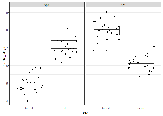
Here we can see that species 2 has larger home ranges on average than species 1, but males in species 1 have larger ones than females while the opposite is true in species 2.
Now let’s see how that translates to our model output.
mod_spp <- lm(home_range ~ sex * species, data = df2)
summary(mod_spp)
##
## Call:
## lm(formula = home_range ~ sex * species, data = df2)
##
## Residuals:
##      Min       1Q   Median       3Q      Max
## -1.15970 -0.28385 -0.02066  0.30467  1.03341
##
## Coefficients:
##                    Estimate Std. Error t value Pr(>|t|)
## (Intercept)         4.98333    0.09187   54.24   <2e-16 ***
## sexmale             2.06773    0.12992   15.91   <2e-16 ***
## speciessp2          3.02179    0.12992   23.26   <2e-16 ***
## sexmale:speciessp2 -3.93157    0.18373  -21.40   <2e-16 ***
## ---
## Signif. codes:  0 '***' 0.001 '**' 0.01 '*' 0.05 '.' 0.1 ' ' 1
##
## Residual standard error: 0.4593 on 96 degrees of freedom
## Multiple R-squared:  0.8603, Adjusted R-squared:  0.8559
## F-statistic: 197.1 on 3 and 96 DF,  p-value: < 2.2e-16
As with before, we can write out the y = mx + b equation:
home_range = msex *sexmale + mspecies *speciessp2 + minteraction *sexmale*speciessp2 + intercept
And fill in the actual coefficient values:
home_range = 2.07*sexmale + 3.02*speciessp2 - 3.93*sexmale*speciessp2 + 4.98
And just as before, we can plug in 1s and 0s into each term depending on whether we have female (0) or male (1) lizards and whether they’re species1 (0) or species2 (1). Since there are only 4 possible combinations of these levels, we can really quickly figure out the means for each group just from skimming the coefficient estimates.
- For females of species 1, only the intercept remains (4.98)
- For males of species 1, the intercept and the sex term remain (4.98 + 2.07)
- For females of species 2, the intercept and the species term remain (4.98 + 3.02)
- For males of species 2, all terms remain (4.98 + 2.07 + 3.02 - 3.93)
In this case, our intercept lizard is a female lizard of species 1. Therefore, the intercept estimate of ~5 makes sense because that’s what we set the mean value of females of this species to when we generated the data. Since we generated males of species 1 with a mean of 7, the sex effect of 2 is intuitive - a male lizard of species 1 would get the intercept term of 5 plus this sex effect of 2. We generated females of species 2 with a mean of 8, so the species effect of 3 is intuitive as well once we add it to the intercept of 5. Finally, for males of species 2, we add the effects of sex and species; however, that assumes that the relationship between males and females is constant across species, which we know is untrue. Therefore adding the interaction term allows this relationship to vary across species.
A reminder about dummy variables
So far, we’ve only used categorical variables with two levels, which makes them very simple to interpret. However, as long as you have a clear understanding of how dummy variables work, then you’ll be able to interpret your model output easily regardless of how many levels your categorical variables have.
When you only have two levels, one level (the first alphabetically, unless you tell R otherwise) will be treated as the intercept, or 0 (sp1 in the previous case) and the other will be treated as the second level, or 1 (sp2 in the previous case). This means that if you have an individual of the first level, the coefficient for that variable reduces to 0, and if you have an individual of the second level, you have an effect of the magnitude of the coefficient. If you are unsure of the order of your levels, look at the coefficient name - it will have the name of the variable AND the name of the level that is coded as a 1 (e.g. “speciessp2” as in our example).
When you add in a third level, you don’t code it as a 2. That type of framework would essentially treat your factor as an integer and assume a linear relationship between the levels – with the third level having double the effect size of the second level – which would not make sense. Instead, we create a second dummy variable. We still treat one level as the intercept value (e.g. sp1), but now we have two coefficients, one associated with each other level (e.g. sp2 and sp3).
home_range = mspecies2 *speciessp2 + mspecies3 *speciessp3 + intercept
For any observation at the second level (e.g. sp2), we could code it as a 1 for the speciessp2 term, but as a 0 for the speciessp3 term. For any observation at the third level (e.g. sp3), we could code it as a 0 for the speciessp2 term, but as a 1 for the speciessp3 term.
We’ll also end up with a second interaction term for this additional level of the categorical variable. Let’s see how this looks if we add a third species to our dataset.
#create a new df
set.seed(123)
df3 <- tibble(species = c(rep("sp1", 50), rep("sp2", 50), rep("sp3", 50)),
              sex = c(rep("female", 25), rep("male", 25),
                      rep("female", 25), rep("male", 25),
                      rep("female", 25), rep("male", 25)),
              home_range = c(rnorm(25, mean = 5, sd = 0.5),
                             rnorm(25, mean = 7, sd = 0.5),
                             rnorm(25, mean = 8, sd = 0.5),
                             rnorm(25, mean = 6, sd = 0.5),
                             #add in new data for a third species with the same means as females from sp1
                             rnorm(25, mean = 5, sd = 0.5),
                             rnorm(25, mean = 5, sd = 0.5)))
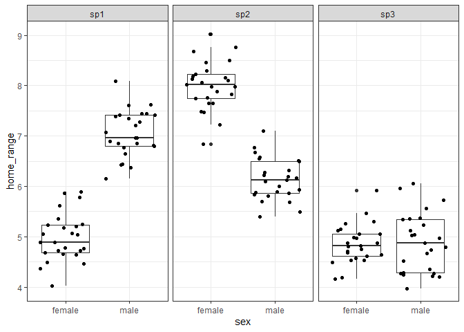
We can see below that this third species now has approximately the same mean home range size for both males and females as our intercept level (females of species 1).
mod_spp3 <- lm(home_range ~ sex * species, data = df3)
summary(mod_spp3)
##
## Call:
## lm(formula = home_range ~ sex * species, data = df3)
##
## Residuals:
##      Min       1Q   Median       3Q      Max
## -1.15970 -0.29350 -0.02066  0.29218  1.16555
##
## Coefficients:
##                    Estimate Std. Error t value Pr(>|t|)
## (Intercept)         4.98333    0.09463   52.66   <2e-16 ***
## sexmale             2.06773    0.13383   15.45   <2e-16 ***
## speciessp2          3.02179    0.13383   22.58   <2e-16 ***
## speciessp3         -0.12174    0.13383   -0.91    0.365
## sexmale:speciessp2 -3.93157    0.18926  -20.77   <2e-16 ***
## sexmale:speciessp3 -2.04483    0.18926  -10.80   <2e-16 ***
## ---
## Signif. codes:  0 '***' 0.001 '**' 0.01 '*' 0.05 '.' 0.1 ' ' 1
##
## Residual standard error: 0.4732 on 144 degrees of freedom
## Multiple R-squared:  0.8711, Adjusted R-squared:  0.8667
## F-statistic: 194.7 on 5 and 144 DF,  p-value: < 2.2e-16
Since all of our coefficient estimates are being compared against our “intercept lizard”, you’ll notice that the estimates for males, species 2, and the interaction between males and species 2 stay roughly the same, even with this new species added to the model. The two new terms are quite easy to interpret then.
- speciessp3 is around 0 and not significant, because females of this species don’t appear to differ from females of species 1
- sexmale:speciessp3 is ~ -2, which essentially counteracts the +2 effect of the coefficient for males. Since the coefficient sexmale is 2, this means that males have larger home ranges than females at our intercept level of species (species 1), but when we look at males from species 3, we actually expect no difference between them and the females.
Two continuous variables
Ok, this is the trickiest one to interpret for sure and in general when you have two continuous variables you should always plot them! But we can still find ways to figure out a general picture of what’s going on without the plots.
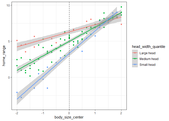
Let’s say we’re still interested in home range size of lizards, but instead of sex or species, we want to know how body size and head width impact home range. Again, we are the lizard god here, so we’re going to create a dataset based on the assumption that larger lizards have bigger home ranges than small lizards, and that larger head widths are correlated with larger home range sizes in larger lizards but not smaller ones.
              #come up with a range of body sizes, repeated 4 times
              #we'll makre sure to center the data too
df4 <- tibble(body_size_center = scale(rep(seq(from = 4, to = 8, length.out = 25),4),
                                scale = FALSE),
              #for each of those 4 sequences, make some random data from low
              #values to high values, so we know that we have a good mix of
              #small to large head sizes with small to large body sizes
              #center the data as well
              head_width_center = scale(c(rnorm(25, mean = 1, sd = 0.5),
                             rnorm(25, mean = 1.5, sd = 0.5),
                             rnorm(25, mean = 2, sd = 0.5),
                             rnorm(25, mean = 2.5, sd = 0.5)), scale = FALSE),
              #create some random noise to scatter around our homerange equation
              noise = rnorm(100, mean = 0, sd = 0.5),
              #make an equation with a strong effect of body size and weak effect
              #of head width, with a positive interaction
              home_range = 5 + 2*body_size_center + 1.5*head_width_center + 1*body_size_center*head_width_center + noise,
              #split body size into quantiles for plotting
              body_size_quantile =
                case_when(body_size_center < (mean(body_size_center) -
                                                sd(body_size_center)) ~ "Small body",
                          body_size_center > (mean(body_size_center) +
                                                sd(body_size_center)) ~ "Large body",
                          TRUE ~ "Medium body"),
              #split head width into quantiles for plotting
              head_width_quantile =
                case_when(head_width_center < (mean(head_width_center) -
                                                 sd(head_width_center)) ~ "Small head",
                          head_width_center > (mean(head_width_center) +
                                                 sd(head_width_center)) ~ "Large head",
                          TRUE ~ "Medium head"))
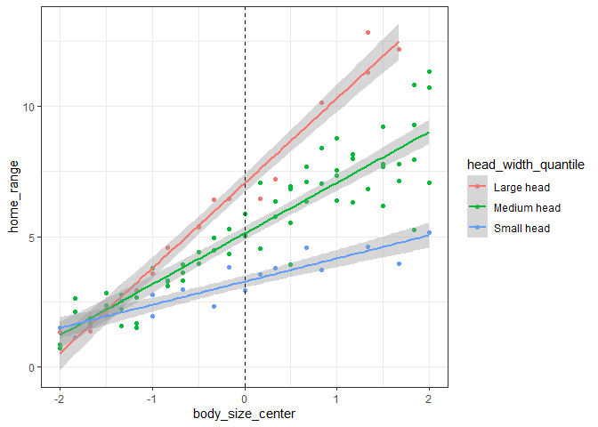
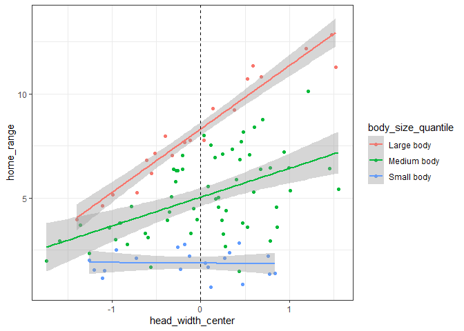
Here, we can see that there is a positive effect of body size across all head widths, but that the effect is a little bit smaller for lizards with smaller heads.
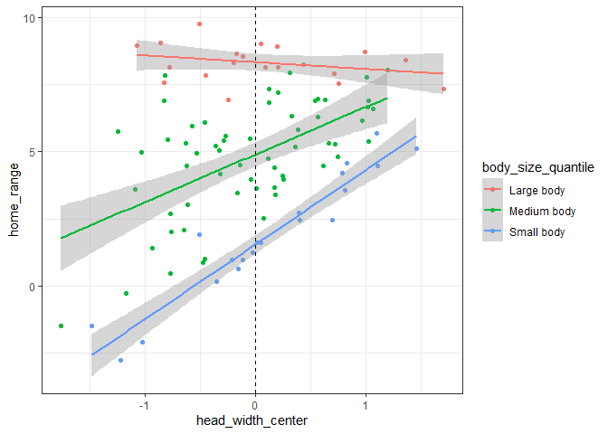
And here we can see that on average there is a small positive effect of head width on home range size, but that for small lizards there is no effect.
When we run our model, we can see that the coefficient estimates are almost identitcal to the values we used to generate the home range data above.
mod_cont <- lm(home_range ~ body_size_center * head_width_center, data = df4)
summary(mod_cont)
##
## Call:
## lm(formula = home_range ~ body_size_center * head_width_center,
##     data = df4)
##
## Residuals:
##      Min       1Q   Median       3Q      Max
## -1.47323 -0.29645  0.01444  0.32346  1.10567
##
## Coefficients:
##                                    Estimate Std. Error t value Pr(>|t|)
## (Intercept)                         5.05388    0.04975  101.58   <2e-16 ***
## body_size_center                    1.96169    0.04154   47.23   <2e-16 ***
## head_width_center                   1.57225    0.06760   23.26   <2e-16 ***
## body_size_center:head_width_center  0.97485    0.05782   16.86   <2e-16 ***
## ---
## Signif. codes:  0 '***' 0.001 '**' 0.01 '*' 0.05 '.' 0.1 ' ' 1
##
## Residual standard error: 0.497 on 96 degrees of freedom
## Multiple R-squared:  0.9692, Adjusted R-squared:  0.9683
## F-statistic:  1008 on 3 and 96 DF,  p-value: < 2.2e-16
Let’s write out our y = mx + b statement again:
home_range = mbody_size *body_size_center + mhead_width*head_width_center + minteraction *body_size_center*head_width_center + intercept
And again with the actual coeffcient values:
home_range = 1.96*body_size_center + 1.57*head_width_center + 0.97*body_size_center*head_width_center + 5.05
Our “intercept lizard” here is a lizard with the mean body size and mean head width (since we centered both variables). We can now interpret the coefficients:
- The intercept is the expected home range size for a lizard with mean
values for both variables
- This corresponds to where the green line intersects 0 in both plots above
- The body size coefficient
represents the expected change in home range size for each cm
increase in body size at the mean head width
- This represents the slope of the green line on the first figure above
- The head width coefficient
represents the expected change in home range size for each cm
increase in head width at the mean body size
- This represents the slope of the green line on the second figure above
- The interaction coefficient tells
us how much each variable impacts the other in their respective
effects on home range size. We can interpret this in two ways:
- For every cm increase in body size, we can expect the effect of head width on home range size to increase by 1 (e.g. for lizards with a body size 1cm greater than the mean body size, the slope of the relationship between head width and home range will increase by 1 relative to the green line above)
- For every cm increase in head width, we can expect the effect of body size on home range size to increase by 1 (e.g. for lizards with a head width 1cm greater than the mean head width, the slope of the relationship between body size and home range will will increase by 1 relative to the green line above)
Therefore, we can see that a positive interaction tells us that the two variables have a synergistic effect – increasing both variables simultaneously results in a much larger effect size than if we simply added the main effects of each variable together. Conversely, a negative interaction tells us that the two variables have an antagonistic effect – increasing both variables simultaneously results in a smaller effect size than if we added the main effects of each together. Below, we can see how this relationship would change in our example if we changed the interaction effect to -1:
As we can see, increasing the value of one variable decreases the effect (i.e. slope of the relationship between dependent and independent variables) of the other variable.
Some final thoughts
Congrats on making it to the end! Hopefully by now you have some helpful tools and visualizations for how interactions work, and over time you’ll be able to quickly understand model outputs without even needing to plot them! Keep in mind that these tips do work for GLM(M)s too, but the linear output you see for your model coefficients will need to be back-transformed out of link space before you explain your results.
You did it!!